TinyGrad MNIST Training and Prediction

Friday. January 17, 2025 - 11 mins

👋 Hello AI enthusiasts! Today we’ll explore how to train a neural network on the MNIST dataset using TinyGrad - the tiny but mighty ML framework! This is part of our journey learning TinyGrad 🚀

📦 Source Code: You can find the complete implementation on GitHub

This project wraps the official TinyGrad MNIST tutorial in a user-friendly interface with ability to save and load models, and to predict on custom images.

Note: This guide is based on TinyGrad’s master branch as of January 17th, 2025 . Windows support for TinyGrad is still limited at this time, which is why we recommend using WSL for Windows users.

Prerequisites and running the project 🛠️

Before we dive in, let’s set up our environment properly:

Windows Users: TinyGrad’s dependencies don’t fully support Windows. We recommend using WSL:
wsl --install
More details at Microsoft’s WSL Guide

Environment Setup 🔧

Create and activate virtual environment:

python -m venv tiny-venv
source tiny-venv/bin/activate  # Linux/WSL

Install dependencies:
```
pip install -r requirements.txt
```

Dependencies used:

tinygrad>=0.7.0    # Core ML framework
numpy>=1.24.0      # Array operations
opencv-python>=4.8.0  # Image processing
colorama>=0.4.6    # Colored terminal output

Install required tools:

sudo apt update && sudo apt full-upgrade --auto-remove
sudo apt install clang nvidia-cuda-toolkit  # For CPU/GPU inference

Place custom images in the pics/ directory for prediction!

Run the project:

python main.py  # This will start the interactive CLI

Code Structure 📁

Our project is organized into:

tinygrad-mnist/
├── model.py         # Neural network architecture
├── data.py          # Dataset handling
├── training.py      # Training logic
├── predict.py       # Prediction interface
├── display.py       # GUI components
└── main.py          # Main application

Project Features ✨

Our implementation includes:

🖼️ Interactive CLI interface with colored output
💾 Model saving and loading with metadata
🔄 Custom image prediction with confidence scores
⏱️ Training time tracking and progress bars
📊 Real-time accuracy metrics
🚀 JIT-compiled training for speed
🖌️ Advanced image preprocessing
🤖 LeNet-5 inspired architecture
💡 Cross-platform terminal support

Interactive Features 🎮

Our project provides a rich interactive experience:

Model Management:
- Load existing models with their training history
- Train new models from scratch
- Auto-save models with timestamps and accuracy

Training Interface:

# Real-time progress tracking
print_progress_bar(iteration, total, length=50)
print_stats(step, loss, acc, best_acc, elapsed_time,num_steps)

Prediction Mode:
- Support for PNG/JPG images
- Batch prediction option
- Confidence scores for predictions
- Interactive file selection

Performance Optimization 🚀

We use TinyGrad’s JIT compilation for faster training:

# JIT compile training step
jit_step = TinyJit(step_fn)
timings = timeit.repeat(jit_step, repeat=5, number=1)
print(f"Best timing: {min(timings) * 1000:.1f}ms")

Model Management 💾

We save models with comprehensive metadata:

training_info = {
    "best_accuracy": stats.best_acc,
    "training_time": str(stats.get_elapsed_time()),
    "total_steps": len(stats.history),
    "batch_size": BATCH_SIZE,
    "device": str(Device.DEFAULT),
    "history": stats.history,
    "num_parameters": len(params)
}

Data Loading 📊

We use TinyGrad’s built-in MNIST dataset loader:

def load_data():
    """Downloads and prepares MNIST dataset for training."""
    print("Loading MNIST dataset...")
    X_train, Y_train, X_test, Y_test = mnist()
    print(f"✓ Loaded dataset with shapes: {X_train.shape}, {Y_train.shape}")
    return X_train, Y_train, X_test, Y_test

Terminal UI 🎨

Our project features a clean terminal interface:

def print_header(batch_size, num_steps):
    """Print training configuration header"""
    print("=" * 60)
    print("MNIST Training with TinyGrad".center(60))
    print("=" * 60)
    print(f"Device: {Device.DEFAULT}")
    print(f"Batch Size: {batch_size}")
    print(f"Total Steps: {num_steps}")

def print_progress_bar(iteration, total, length=50):
    """Show real-time training progress"""
    filled = int(length * iteration // total)
    bar = "█" * filled + "░" * (length - filled)
    percent = f"{100 * iteration / total:.1f}%"
    return f"[{bar}] {percent}"

Model Architecture 🧠

We use a LeNet-5 inspired CNN architecture, carefully designed for the MNIST digit recognition task. Here’s a detailed breakdown of each layer:

class Model:
    def __init__(self):
        # Conv1: Input → First Feature Extraction
        # - Input: 1 channel (grayscale) 28x28 image
        # - Output: 32 feature maps of size 26x26
        # - 3x3 kernel learns local patterns like edges and curves
        self.l1 = nn.Conv2d(1, 32, kernel_size=(3, 3))

        # Conv2: Feature Refinement
        # - Input: 32 channels of 13x13 (after maxpool)
        # - Output: 64 deeper features of size 11x11
        # - 3x3 kernel combines features into more complex patterns
        self.l2 = nn.Conv2d(32, 64, kernel_size=(3, 3))

        # Fully Connected: Classification
        # - Input: 1600 flattened features (64 * 5 * 5 after maxpool)
        # - Output: 10 classes (digits 0-9)
        # - Dropout(0.5) prevents overfitting
        self.l3 = nn.Linear(1600, 10)

    def __call__(self, x):
        # Block 1: Initial Feature Extraction
        # MaxPool reduces spatial dimensions by 2x while keeping important features
        x = self.l1(x).relu().max_pool2d((2, 2))  # 28x28 → 13x13

        # Block 2: Advanced Feature Learning
        # Second pooling further reduces dimensions
        x = self.l2(x).relu().max_pool2d((2, 2))  # 13x13 → 5x5

        # Classification Block
        # Flatten → Dropout → Linear transformation
        return self.l3(x.flatten(1).dropout(0.5))

Key architectural decisions:

Two Convolutional Layers: Progressive feature extraction from simple to complex patterns
ReLU Activation: Introduces non-linearity and prevents vanishing gradients
Max Pooling: Reduces spatial dimensions while retaining important features
Dropout: Prevents overfitting by randomly deactivating 50% of neurons during training
Fully Connected Layer: Final classification layer with softmax activation (implicit)

This architecture achieves ~99% accuracy on the MNIST test set while remaining computationally efficient.

Training Pipeline 🎯

Our training setup includes:

# Hyperparameters
BATCH_SIZE = 128
NUM_STEPS = 7000
EVAL_INTERVAL = 100

# Training stats tracker
class TrainingStats:
    def __init__(self):
        self.best_acc = 0.0
        self.start_time = datetime.now()
        self.history = []

Model Persistence 💾

We save both model weights and training info:

def save_model(model, stats):
    # Save weights in safetensors format
    safe_save(param_dict, "weights.safetensors")
    
    # Save training metadata
    training_info = {
        "best_accuracy": stats.best_acc,
        "training_time": str(stats.get_elapsed_time()),
        "device": str(Device.DEFAULT),
        "history": stats.history,
        "num_parameters": len(params)
    }

Prediction Interface 🔮

Our prediction system includes sophisticated image preprocessing:

def load_and_preprocess_image(image_path):
    """Prepare any image for MNIST prediction"""
    # Load grayscale image
    img = cv2.imread(image_path, cv2.IMREAD_GRAYSCALE)
    
    if not is_mnist_format(img):
        # Enhance contrast
        img = cv2.normalize(img, None, 0, 255, cv2.NORM_MINMAX)
        
        # Convert to black & white
        _, img = cv2.threshold(img, 127, 255, cv2.THRESH_BINARY + cv2.THRESH_OTSU)
        
        # Find & crop digit
        coords = cv2.findNonZero(255 - img)
        x, y, w, h = cv2.boundingRect(coords)
        
        # Add padding & make square
        img = add_padding_and_square(img[y:y+h, x:x+w])
        
        # Resize to MNIST format (28x28)
        img = cv2.resize(img, (28, 28))
    
    return Tensor(img.reshape(1, 1, 28, 28))

Interactive CLI 💻

We provide a user-friendly command-line interface:

def predict_local_images(model):
    """Predict digits from local PNG/JPG files"""
    while True:
        # List available images
        image_files = glob.glob("pics/*.{png,jpg}")
        
        # Show options
        print("1-N. Select image to predict")
        print("a. Predict all images")
        print("q. Quit")
        
        # Make prediction with confidence
        prediction = model(img_tensor).argmax().item()
        confidence = model(img_tensor).softmax()[0][prediction].item()
        print(f"Predicted: {prediction} (Confidence: {confidence:.2f})")

Visual Walkthrough 📸

Let’s see the project in action:

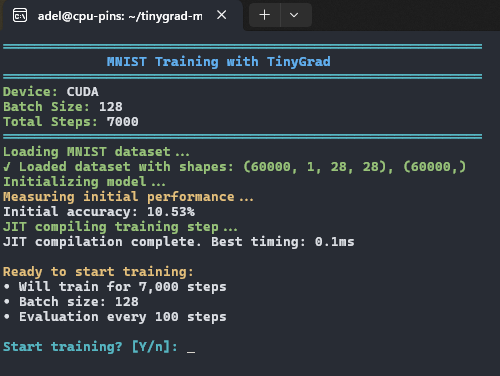
1. Initial Setup

Initial TUI Info

The clean terminal interface shows system info and training configuration

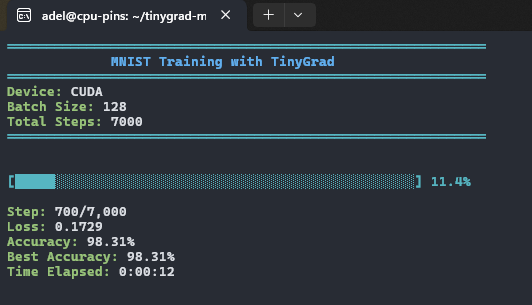
2. Training Progress

Training Progress

Real-time training progress with accuracy metrics and progress bar

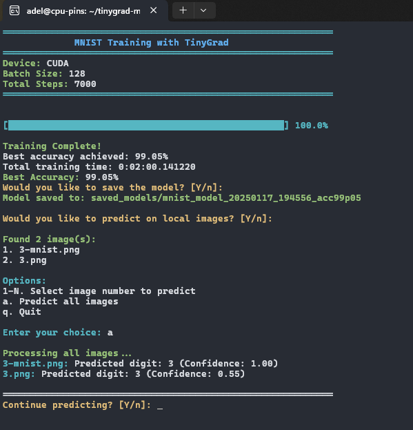
3. Prediction Interface

Prediction Results

Making predictions on custom digit images with confidence scores

Real-World Performance Examples 🎯

Let’s examine how our model performs on different types of inputs:

MNIST Test Sample

MNIST Sample Prediction

Prediction on a standard MNIST test sample - 100% confidence on digit 3

Hand-Drawn Sample

Hand-Drawn Sample Prediction

Prediction on a hand-drawn digit - Correctly identified as 3 with 55% confidence

This comparison highlights an important aspect of machine learning models: while they achieve high confidence on data similar to their training set (MNIST samples), they show lower but still reasonable confidence on real-world inputs that may differ in style, stroke width, or exact positioning. This is expected behavior and demonstrates both the model’s capabilities and limitations in real-world applications.

Adel Aloui

Software Engineer with expertise in building innovative AI-driven solutions.